Procedural Volumetric Clouds
03 May 2023Volumetric clouds use 3D density functions to represent clouds in a realistic way. Ray marching is used to generate photorealistic rendering. With modern graphics cards it is possible to do this in realtime.
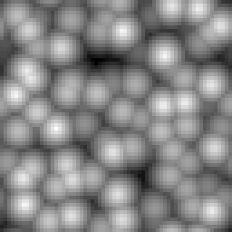
Sebastian Lague’s video on cloud rendering shows how to generate Worley noise which can be used to generate realistic looking clouds. Worley noise basically is a function which for each location returns the distance to the nearest point of a random set of points. Usually the space is divided into cells with each cell containing one random point. This improves the performance of determining the distance to the nearest point. The following image shows a slice through inverted 3D Worley noise.
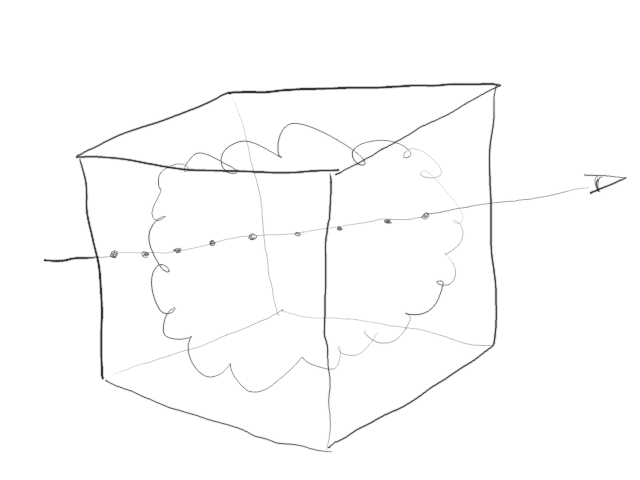
Ray marching works by starting a view ray for each render pixel and sampling the cloud volume which is a cube in this example. This ray tracing program can be implemented in OpenGL by rendering a dummy background quad.
The transmittance for a small segment of the cloud is basically the exponent of negative density times step size:
vec3 cloud_scatter = vec3(0, 0, 0);
float transparency = 1.0;
for (int i=0; i<cloud_samples; i++) {
vec3 c = origin + (i * stepsize + 0.5) * direction;
float density = cloud_density(c);
float transmittance_cloud = exp(-density * stepsize);
float scatter_amount = 1.0;
cloud_scatter += transparency * (1 - transmittance_cloud) * scatter_amount;
transparency = transparency * transmittance_cloud;
};
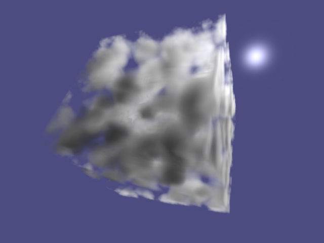
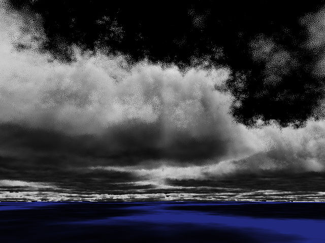
incoming = incoming * transparency + cloud_scatter;The resulting sampled cube of Worley noise looks like this:

The amount of scattered light can be changed by using a mix of isotropic scattering and a phase function for approximating Mie scattering. I.e. the amount of scattered light is computed as follows:
float scatter_amount = anisotropic * phase(0.76, dot(direction, light_direction)) + 1 - anisotropic;I used the Cornette and Shanks phase function shown below (formula (4) in Bruneton’s paper):
float M_PI = 3.14159265358;
float phase(float g, float mu)
{
  return 3 * (1 - g * g) * (1 + mu * mu) / (8 * M_PI * (2 + g * g) * pow(1 + g * g - 2 * g * mu, 1.5));
}
The resulting rendering of the Worley noise now shows a bright halo around the sun:

The rendering does not yet include self-shadowing. Shadows are usually computed by sampling light rays towards the light source for each sample of the view ray. However a more efficient way is to use deep opacity maps (also see Pixar’s work on deep shadow maps). In a similar fashion to shadow maps, a depth map of the start of the cloud is computed as seen from the light source. While rendering the depth map, several samples of the opacity (or transmittance) behind the depth map are taken with a constant stepsize. I.e. the opacity map consists of a depth (or offset) image and a 3D array of opacity (or transmittance) images.

Similar as when performing shadow mapping, one can perform lookups in the opacity map to determine the amount of shading at each sample in the cloud.

To make the cloud look more realistic, one can add multiple octaves of Worley noise with decreasing amplitude. This is also sometimes called fractal Brownian motion.
To reduce sampling artifacts without loss of performance, one can use blue noise offsets for the sample positions when computing shadows as well as when creating the final rendering.

In a previous article I have demonstrated how to generate global cloud cover using curl noise. One can add the global cloud cover with octaves of mixed Perlin and Worley noise and subtract a threshold. Clamping the resulting value creates 2D cloud patterns on a spherical surface.

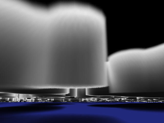
By restricting the clouds to be between a bottom and top height, one obtains prism-like objects as shown below:
Note that at this point it is recommended to use cascaded deep opacity maps instead of a single opacity map. Like cascaded shadow maps, cascaded deep opacity maps are a series of cuboids covering different splits of the view frustum.
One can additionally multiply the clouds with a vertical density profile.

Guerilla Games uses a remapping function to introduce high frequency noise on the surfaces of the clouds. The high frequency noise value is remapped using a range defined using the low frequency noise value.
float density = clamp(remap(noise, 1 - base, 1.0, 0.0, cap), 0.0, cap);The remapping function is defined as follows:
float remap(float value, float original_min, float original_max, float new_min, float new_max)
{
  return new_min + (value - original_min) / (original_max - original_min) * (new_max - new_min);
}
The function composing all those noise values is shown here:
uniform samplerCube cover;
float cloud_density(vec3 point, float lod)
{
  float clouds = perlin_octaves(normalize(point) * radius / cloud_scale);
  float profile = cloud_profile(point);
  float cover_sample = texture(cover, point).r * gradient + clouds * multiplier - threshold;
  float base = cover_sample * profile;
  float noise = cloud_octaves(point / detail_scale, lod);
  float density = clamp(remap(noise, 1 - base, 1.0, 0.0, cap), 0.0, cap);
  return density;
}
See cloudsonly.clj for source code.
An example obtained using these techniques is shown below:
The example was rendered with 28.5 frames per second.
- an AMD Ryzen 7 4700U with passmark 2034 was used for rendering
- the resolution of the render window was 640x480
- 3 deep opacity maps with one 512x512 offset layer a 7x512x512 transmittance array were rendered for each frame
- 5 octaves of 64x64x64 Worley noise were used for the high frequency detail of the clouds
- a vertical profile texture with 10 values was used
- 3 octaves of 64x64x64 Perlin-Worley noise were used for the horizontal 2D shapes of the clouds
- a 6x512x512 cubemap was used for the global cloud cover
Please let me know any suggestions and improvements!
![]()
Enjoy!
Update: I removed the clamping operation for the cover sample noise.
Update: Implementing the powder sugar effect is actually quite simple.
Essentially the increment to the scattered light by the cloud is multiplied with powder(density * stepsize) where the powder function is defined as follows:
uniform float powder_decay;

float powder(float d)
{
  return 1.0 - exp(-powder_decay * d);
}
The fact that there is less light to be scattered at the fringe of a cloud is approximated by reducing the amount of scattered light in low density areas of the cloud.
Future work
- add atmospheric scattering with cloud shadows
- add planet surface and shadow map
- sampling with adaptive step size
- problems with shadow map at large distances
- problem with long shadows at dawn