The Clojure programming language has desirable properties for software engineering such as immutability and strong support for implementing parallel algorithms.
Currently Python is popular for machine learning due to Pytorch and other machine learning libraries targeting the Python programming language.
However using libpython-clj2 one can invoke Pytorch for machine learning from within Clojure.
This article demonstrates a few basics of machine learning using the \(y=x^2\) parabola function as an example.
Import PyTorch
The PyTorch library is quite comprehensive, is free software, and you can find a lot of documentation on how to use it.
The default version of PyTorch on pypi.org comes with CUDA (Nvidia) GPU support.
There are also PyTorch wheels provided by AMD which come with ROCm support.
Here we are going to use a CPU version of PyTorch which is a much smaller install.
You need to install Python 3.10 or later.
For package management we are going to use the uv package manager.
The following pyproject.toml file is used to install PyTorch and NumPy.
Note that we are specifying a custom repository index to get the CPU-only version of PyTorch.
Also we are using the system version of Python to prevent uv from trying to install its own version which lacks the _cython module.
To freeze the dependencies and create a uv.lock file, you need to run
uv lock
You can install the dependencies using
uv sync
In order to access PyTorch from Clojure you need to run the clj command via uv:
uv run clj
Now you should be able to import the Python modules using require-python.
development data is used to check that the model is not overfitting or underfitting
test data is used to report the performance of the model
Next we are going to use PyTorch DataLoaders to split training and development data into mini-batches.
The data loaders are also used to shuffle the data sets.
Shuffling can be quite important for stability of the training process.
Each arrow represents a weight stored in the fully connected layers fc1, fc2, and fc3.
There are different layer types in PyTorch.
A fully connected layer is the most basic one.
To be able to model non-linear functions, activation functions are used (here: sigmoid).
The model looks like this when using 8 units in each hidden layer.
When evaluating a model, you should disable gradient accumulation.
Otherwise gradients will leak into subsequent training steps.
In Python this looks like this:
withtorch.no_grad():...
In Clojure we can define a macro to disable gradient accumulation:
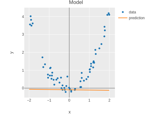
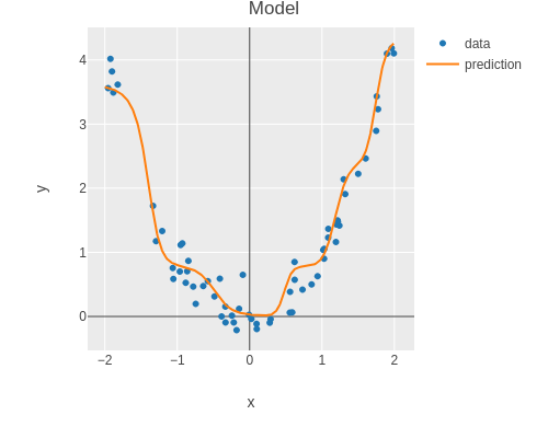
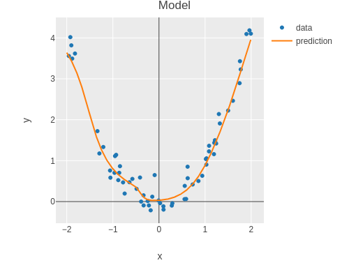
Before training, the model should just be a random function.
(plot-modelfeatureslabelsmodel)
Using the test set, we can report the performance of the model.
Note that it is good practice to use a separate test set to report performance, because hyperparameter tuning using the dev set can overfit the model to the dev set.
Note that the output is not zero.
PyTorch performs random initialisation of the weights for us.
Breaking the symmetry like this is important, otherwise all activations and gradients will be the same and the model will not be able to learn.
Training
A training epoch performs the following step for each mini-batch in the training set:
reset the gradient of the optimizer
perform model predictions for the input features
compute the loss which compares the predictions with the labels
perform backpropagation to get gradients for each model parameter
perform a gradient descent step using the optimizer
In order to check whether the model is overfitting or underfitting, we need to evaluate the model on the development set.
The following method computes the loss values for each mini-batch in the development set.
Now we can implement a training run.
A training run basically consists of many training epochs.
Here we are using the stochastic gradient descent method (SGD).
Note that usually the Adam optimizer is used, because it is more efficient.
As a loss function we simply use the mean squared error (MSE).
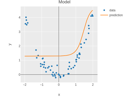
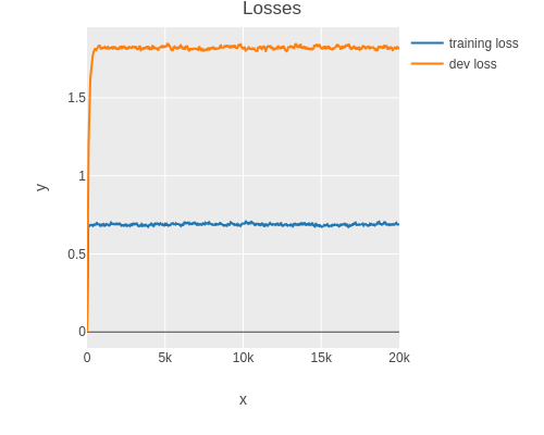
As one can see, the model is overfitting the training set.
I.e. the model fits the training data closely but does not generalize well.
This makes the model sensitive to noise.
Here one can observe overfitting directly.
In general however one uses the training and dev loss to detect if the model is overfitting.
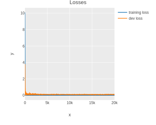
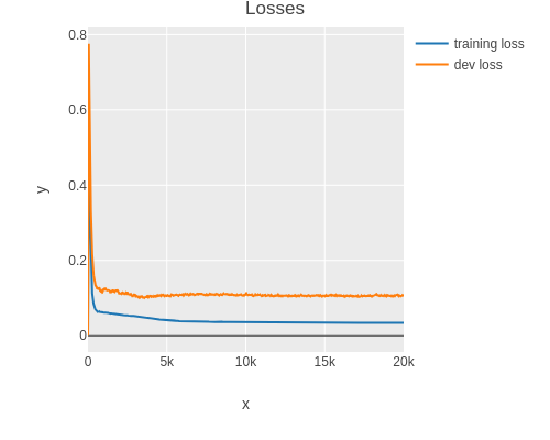
First we define a smoothing function which smoothes a sequence of loss values.
As one can see, the final dev set loss is more than twice the amount of the training loss.
This is a sign that the model is overfitting (high variance).
High variance can be resolved using the following techniques:
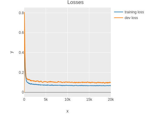
Instead of tuning the number of hidden units and layers (which can only be done in discrete steps), one can use regularization.
Here we are using dropout regularization which randomly sets some activations to zero during training.
After trying out a few values, I found 0.05 to be a good dropout rate for this dataset size and model.
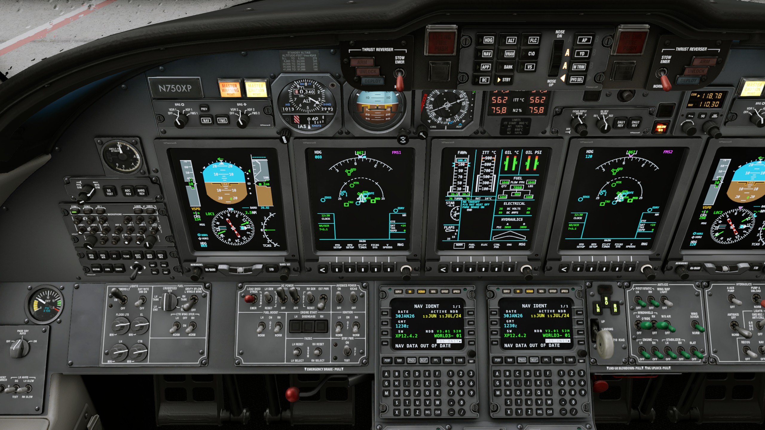
If you are trying out the Citation-X with X-Plane 12, I can really recommend the XChecklist plugin and the checklist file for the Citation-X.
To help you with finding all the different controls, I created this interactive page.
PRELIMINARY
Aircraft Doors: OPEN
Parking Brake: SET
Landing Gear Handle: DOWN
Speedbrake Handle: CHECK ZERO
Throttles: CUT OFF
Battery Switches 1 & 2: ON
Eicas Switch: ON
Battery Volts (Elec Page): CHECK 24
Refuel: AS NEEDED
Fuel Balance: CHECK IMBALANCE <200 lbs
Eicas Switch: OFF
Battery Switches 1 & 2: OFF
Standby Power: TEST
Passengers & Cargo: BOARDED & CHECK
COCKPIT PREPARATION 1
Battery Switches 1 & 2: ON
External Power if Available: ON
Left & Right Generator: UP
Eicas Switch: ON
Avionics Switch: ON
Fuel Boost: BOTH NORM or ON
FADEC Left Switch: RESET & NORMAL
FADEC Right Switch: RESET & NORMAL
Ignition Switches: CHECK NORM
Standby Power: ON
Center Wing Transfer: BOTH NORM
Emergency Exit Lights: ON (Red Light On)
Emergency Exit Lights: ARM
Instrument Lights (FLOOD LTS, EL, LH, CTR): SET AS NEED
Passenger Oxygen: AUTO
Master Warning: RESET
Master Caution: RESET
Windshield Heater LH & RH: ON
COCKPIT PREPARATION 2
Aux Pump A: ON
Parking Brake: OFF
Parking Brake: ON
Aux Pump A: OFF
Seat Belt Lights: UP
Recognition Lights: ON
Navigation Lights: ON
Tail Flood Lights: ON
Engine Bleed Air: BOTH HP/LP
Righthand Panel Lights: SET
APU Master: ON
Test Button: CHECK
APU Start: HOLD TILL START
APU N1: 100 RPM
APU Generator: ON
APU Bleed Air: MAX COOL
Cabin and Cockpit Packs: ON
PREFLIGHT PROCEDURE
Aircraft Doors: CLOSED
External Power if Available: DISCONNECTED
Rotary Test: ROTATE TO ALL POSITIONS
Aux Pump A: ON
Flaps & Slats: RETRACT
Aux Pump A: OFF
PFD Source Selection: SELECT FMS or NAV
Lateral Navigation Mode: NAV
Vertical Navigation Mode: FLC
Flight Level Change Target Airspeed: 180 KIAS
Yaw Damper: ON
Mach Trim: ON
Transponder Frequency: SET
Transponder Mode: STANDBY
Heading: SET TO RUNWAY
Altitude Select: SET TO CLEARED ALT
Altimeter Baro: SET LOCAL QNH
Minimums BARO PFD: SET TO 1000FT AGL
ENGINE START
GND REC/ANTI-COLL Lights: ON
Cabin and Cockpit Packs: OFF
Engine Start RH Button: PRESS
RH N2%: WAIT >10
Right Power Lever: IDLE
RH N2%: WAIT >60
Engine Start LH Button: PRESS
LH N2%: WAIT >10
Left Power Lever: IDLE
Eicas Fuel Page: CHECK FLOW >500 PPH
Eicas Hyd Page: CHECK PSI>3000
Engine Bleed Air: BOTH LP
Cabin and Cockpit Packs: ON
BEFORE TAXI
Pressurization Switches: ALL THREE NORM
Pressurization Altitude: SET
Pitot Static Switches: BOTH UP
Flaps 5 or 15: SET
Pitch Trim: SET GREEN
Rudder & Aileron Trim: CHECK NEUTRAL
Yoke Roll Control: FREE MOVEMENT
Yoke Pitch Control: FREE MOVEMENT
Rudder Control: FREE MOVEMENT
Speedbrake Handle: CHECK MOVEMENT THEN ZERO
Taxi Light: ON
TAXI
Parking Brake: RELEASED
Parking Brake: SET
BEFORE TAKEOFF
GND REC/ANTI-COLL Lights: UP
Landing Lights: ON
Taxi Light: OFF
Transponder: ALT
Parking Brake: RELEASED
Pedal Brakes: FULL PRESS
TAKEOFF
Throttle Lever: SET 40% N1
Both Engines Simultaneous: CHECK
Pedal Brakes: RELEASE
Throttle Lever: MAX POSITION T/O
At Vr Speed: ROTATE
AFTER TAKEOFF
==>: Positive Rating Climb
Landing Gear: UP
==>: Above 1000ft AGl
Autopilot: ENGAGE
Vertical Navigation Mode: FLC or VNAV
Flaps & Slats: UP AS REQUIRED
Throttle Lever: CLB POSITION
Cabin Pressurization: CHECK POSITIVE FPM
Altimeter Baro: STD AT TRANS ALT
==>: Above 10000ft
Landing Lights: OFF
Seat Belt Lights: OFF
APU Bleed Air: OFF
APU Generator: OFF
APU Start: HOLD DOWN
==>: APU RPM ZERO
APU Master: OFF
==>: Above 18000ft
ENG SYNC: FAN
CRUISE
BANK: AS REQUIRED
Throttle Lever: CRU POSITION
DESCENT
Altitude Knob: SET TO CLEARED ALT
Vertical Navigation Mode: SET VNAV, FLC or VS
==>: Below 18000ft
ENG SYNC: OFF
BANK: AS REQUIRED
APU Master: ON
APU Start: HOLD TILL START
APU N1 100%: READY
APU Generator: ON
APU Bleed Air: MAX COOL
==>: Below 10000ft
Landing Lights: ON
Seat Belt Lights: ON
Altimeter Baro: SET LOCAL QNH
RA/BARO Minimums: SET
APPROACH & LANDING
==>: SPEED <250 KIAS
Slats & Flaps: FLAPS 5
Autopilot Approach Mode: ARM
==>: SPEED <210 KIAS
Flaps: FLAPS 15
Landing Gear: DOWN 3 GREEN
==>: SPEED 180 KIAS
Flaps: FLAPS 35
==>: AGL <500 ft
AP & YD: DISCONNECT
Throttle Lever: IDLE
Reverse Throttle: IF NECESSARY
==>: GND SPEED <50 KIAS
Reverse Throttle: OFF
AFTER LANDING
Pitot Static Heat: BOTH OFF
GND REC/ANTI-COLL Lights: GND REC
Transponder Mode: STANDBY
Taxi Light: ON
Landing Lights: OFF
Speedbrakes: RETRACTED
Flaps: UP
SHUTDOWN
Taxi Light: OFF
Parking Brake: SET
Throttles: CUT OFF
Engines N2%: Below 10%
GND REC/ANTI-COLL Lights: OFF
Aircraft Doors: OPEN
Seat Belts: OFF
APU Bleed Air: OFF
APU Generator: OFF
APU Start: HOLD DOWN
==>: APU RPM ZERO
APU Master: OFF
Engine Bleed Air: BOTH OFF
Cabin and Cockpit Packs: OFF
Recognition Lights: OFF
Navigation Lights: OFF
Tail Flood Lights: OFF
Windshield Heater LH & RH: OFF
Passenger Oxygen: OFF
Emergency Exit Lights: OFF
Center Wing Transfer: BOTH OFF
Fuel Boost: BOTH OFF
Standby Power: OFF
Avionics Switch: OFF
Eicas Switch: OFF
Left & Right Generator: OFF
Battery Switches 1 & 2: BOTH OFF
Autopilot explanation
Vertical flight path
FLC: Flight Level Change climbs/descends to the target altitude while keeping the target speed.
VS: Vertical Speed climb/descends to the target altitude using a specified target rate.
VNAV: Vertical Navigation the flight management system (FMS) controls the altitude but never descends below the target altitude.
ALT: Altitude Hold Keep the autopilot at the current altitude. This mode is entered automatically by some of the other modes when the target altitude is reached.
Lateral navigation
HDG: Heading tells the autopilot to turn to the target heading.
NAV: Lateral Navigation uses the flight management system (FMS) or the VOR/ILS for controlling the heading.
Both
APP: Approach arms the ILS approach. The airplane should be below the ILS glide path so that the autopilot can start descending when encountering the glide path.
Other
AP: Engage/Disengage autopilot but keep displaying guidance information.
STBY: Disengage autopilot and clear guidance information.
BANK: Toggle reduced maximum bank angle used by autopilot.
C/O: Change Over switch between displaying airspeed in IAS (Indicated Airspeed in knots) and Mach number. Mach number display is used at high altitudes (e.g. when climbing above 25000 feet (flight level 250)).
BC: Back Course is a legacy mode allowing to use the back course of an old ILS.
Recently I started to look into the problem of reentry trajectory planning in the context of developing the sfsim space flight simulator.
I had looked into reinforcement learning before and even tried out Q-learning using the lunar lander reference environment of OpenAI’s gym library (now maintained by the Farama Foundation).
However it had stability issues.
The algorithm would converge on a strategy and then suddenly diverge again.
More recently (2017) the Proximal Policy Optimization (PPO) algorithm was published and it has gained in popularity.
PPO is inspired by Trust Region Policy Optimization (TRPO) but is much easier to implement.
Also PPO handles continuous observation and action spaces which is important for control problems.
The Stable Baselines3 Python library has a implementation of PPO, TRPO, and other reinforcement learning algorithms.
However I found XinJingHao’s PPO implementation which is easier to follow.
In order to use PPO with a simulation environment implemented in Clojure and also in order to get a better understanding of PPO, I dediced to do an implementation of PPO in Clojure.
Dependencies
For this project we are using the following deps.edn file.
The Python setup is shown further down in this article.
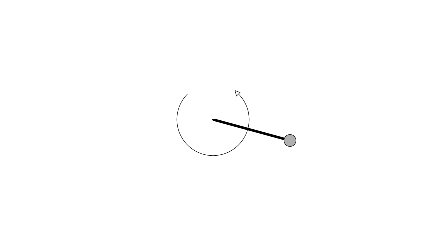
To validate the implementation, we will implement the classical pendulum environment in Clojure.
In order to be able to switch environments, we define a protocol according to the environment abstract class used in OpenAI’s gym.
Same as in OpenAI’s gym the angle is zero when the pendulum is pointing up.
Here a pendulum is initialised to be pointing down and have an angular velocity of 0.5 radians per second.
The motor is controlled using an input value between -1 and 1.
This value is simply multiplied with the maximum angular acceleration provided by the motor.
(defnmotor-acceleration"Angular acceleration from motor"[controlmotor-acceleration](*controlmotor-acceleration))
A simulation step of the pendulum is implemented using Euler integration.
(defnupdate-state"Perform simulation step of pendulum"([{:keys[anglevelocityt]}{:keys[control]}{:keys[dtmotorgravitationlengthmax-speed]}](let[gravity(pendulum-gravitygravitationlengthangle)motor(motor-accelerationcontrolmotor)t(+tdt)acceleration(+motorgravity)velocity(max(-max-speed)(minmax-speed(+velocity(*accelerationdt))))angle(+angle(*velocitydt))]{:angleangle:velocityvelocity:tt})))
Here are a few examples for advancing the state in different situations.
The observation of the pendulum state uses cosinus and sinus of the angle to resolve the wrap around problem of angles.
The angular speed is normalized to be between -1 and 1 as well.
This so called feature scaling is done in order to improve convergence.
(defnobservation"Get observation from state"[{:keys[anglevelocity]}{:keys[max-speed]}][(cosangle)(sinangle)(/velocitymax-speed)])
The observation of the pendulum is a vector with 3 elements.
Note that the observation needs to capture all information required for achieving the objective, because it is the only information available to the actor for deciding on the next action.
Action
The action of a pendulum is a vector with one element between 0 and 1.
The following method clips it and converts it to an action hashmap used by the pendulum environment.
Note that an action can consist of several values.
(defnaction"Convert array to action"[array]{:control(max-1.0(min1.0(-(*2.0(firstarray))1.0)))})
The following examples show how the action vector is mapped to a control input between -1 and 1.
The truncate method is used to stop a pendulum run after a specific amount of time.
(defntruncate?"Decide whether a run should be aborted"([{:keys[t]}{:keys[timeout]}](>=ttimeout)))(truncate?{:t50.0}{:timeout100.0}); false(truncate?{:t100.0}{:timeout100.0}); true
It is also possible to define a termination condition.
For the pendulum environment we specify that it never terminates.
The following method normalizes an angle to be between -PI and +PI.
(defnnormalize-angle"Angular deviation from up angle"[angle](-(mod(+anglePI)(*2PI))PI))
We also need the square of a number.
(defnsqr"Square of number"[x](*xx))
The reward function penalises deviation from the upright position, non-zero velocities, and non-zero control input.
Note that it is important that the reward function is continuous because machine learning uses gradient descent.
With Quil we can create an animation of the pendulum and react to mouse input.
(defn-main[&_args](let[done-chan(async/chan)last-action(atom{:control0.0})](q/sketch:title"Inverted Pendulum with Mouse Control":size[854480]:setup#(setupPI0.0):update(fn[state](let[action{:control(min1.0(max-1.0(-1.0(/(q/mouse-x)(/(q/width)2.0)))))}state(update-statestateactionconfig)](when(done?stateconfig)(async/close!done-chan))(reset!last-actionaction)state)):draw#(draw-state%@last-action):middleware[m/fun-mode]:on-close(fn[&_](async/close!done-chan)))(async/<!!done-chan))(System/exit0))
Neural Networks
PPO is a machine learning technique using backpropagation to learn the parameters of two neural networks.
The actor network takes an observation as an input and outputs the parameters of a probability distribution for sampling the next action to take.
The critic takes an observation as an input and outputs the expected cumulative reward for the current state.
Import PyTorch
For implementing the neural networks and backpropagation, we can use the Python-Clojure bridge libpython-clj2 and the PyTorch machine learning library.
The PyTorch library is quite comprehensive, is free software, and you can find a lot of documentation on how to use it.
The default version of PyTorch on pypi.org comes with CUDA (Nvidia) GPU support.
There are also PyTorch wheels provided by AMD which come with ROCm support.
Here we are going to use a CPU version of PyTorch which is a much smaller install.
You need to install Python 3.10 or later.
For package management we are going to use the uv package manager.
The following pyproject.toml file is used to install PyTorch and NumPy.
Note that we are specifying a custom repository index to get the CPU-only version of PyTorch.
Also we are using the system version of Python to prevent uv from trying to install its own version which lacks the _cython module.
To freeze the dependencies and create a uv.lock file, you need to run
uv lock
You can install the dependencies using
uv sync
In order to access PyTorch from Clojure you need to run the clj command via uv:
uv run clj
Now you should be able to import the Python modules using require-python.
A tensor with no dimensions can also be converted using toitem
(defntoitem"Convert torch scalar value to float"[tensor](py.tensoritem))(toitem(tensorPI)); 3.1415927410125732
Critic Network
The critic network is a neural network with an input layer of size observation-size and two fully connected hidden layers of size hidden-units with tanh activation functions.
The critic output is a single value (an estimate for the expected cumulative return achievable by the given observed state).
When running inference, you need to run the network with gradient accumulation disabled, otherwise gradients get accumulated and can leak into a subsequent training step.
In Python this looks like this.
withtorch.no_grad():# ...
Here we create a Clojure macro to do the same job.
(defmacrowithout-gradient"Execute body without gradient calculation"[&body]`(let[no-grad#(torch/no_grad)](try(py.no-grad#~'__enter__)~@body(finally(py.no-grad#~'__exit__nilnilnil)))))
Now we can create a network and try it out.
We create a test multilayer perceptron with three inputs, two hidden layers of 8 units each, and one output.
(defcritic(Critic38))
Note that the network creates non-zero outputs because PyTorch performs random initialisation of the weights for us.
Training a neural network is done by defining a loss function.
The loss of the network then is calculated for a mini-batch of training data.
One can then use PyTorch’s backpropagation to compute the gradient of the loss value with respect to every single parameter of the network.
The gradient then is used to perform a gradient descent step.
A popular gradient descent method is the Adam optimizer.
The actor network for PPO takes an observation as an input and it outputs the parameters of a probability distribution over actions.
In addition to the forward pass, the actor network has a method deterministic_act to choose the expectation value of the distribution as a deterministic action.
Furthermore the actor network has a method get_dist to return a Torch distribution object which can be used to sample a random action or query the current log-probability of an action.
Here (as the default in XinJingHao’s PPO implementation) we use the Beta distribution with parameters alpha and beta both greater than 1.0.
See here for an interactive visualization of the Beta distribution.
(defnindeterministic-act"Sample action using actor network returning random action and log-probability"[actor](fnindeterministic-act-with-actor[observation](without-gradient(let[dist(py.actorget_dist(tensorobservation))sample(py.distsample)action(torch/clampsample0.01.0)logprob(py.distlog_probaction)]{:action(tolistaction):logprob(tolistlogprob)}))))
We create a test multilayer perceptron with three inputs, two hidden layers of 8 units each, and two outputs which serve as parameters for the Beta distribution.
(defactor(Actor381))
One can then use the network to:
a. get the parameters of the distribution for a given observation.
We can also query the current log-probability of a previously sampled action.
(defnlogprob-of-action"Get log probability of action"[actor](fn[observationaction](let[dist(py.actorget_distobservation)](py.distlog_probaction))))
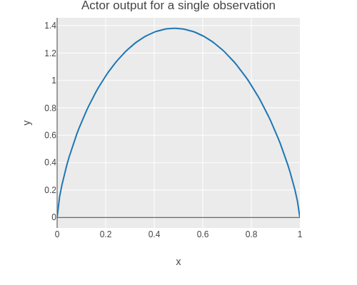
Here is a plot of the probability density function (PDF) actor output for a single observation.
(without-gradient(let[actions(range0.01.010.01)logprob(fn[action](tolist((logprob-of-actionactor)(tensor[-100])(tensoraction))))scatter(tc/dataset{:xactions:y(map(fn[action](exp(first(logprob[action]))))actions)})](->scatter(plotly/base{:=title"Actor output for a single observation":=mode:lines})(plotly/layer-point{:=x:x:=y:y}))))
Finally we can also query the entropy of the distribution.
By incorporating the entropy into the loss function later on, we can encourage exploration and prevent the probability density function from collapsing.
(defnentropy-of-distribution"Get entropy of distribution"[actorobservation](let[dist(py.actorget_distobservation)](py.distentropy)))(without-gradient(entropy-of-distributionactor(tensor[-100]))); tensor([-0.0825])
Proximal Policy Optimization
Sampling data
In order to perform optimization, we sample the environment using the current policy (indeterministic action using actor).
(defnsample-environment"Collect trajectory data from environment"[environment-factorypolicysize](loop[state(environment-factory)observations[]actions[]logprobs[]next-observations[]rewards[]dones[]truncates[]isize](if(pos?i)(let[observation(environment-observationstate)sample(policyobservation)action(:actionsample)logprob(:logprobsample)reward(environment-rewardstateaction)done(environment-done?state)truncate(environment-truncate?state)next-state(if(ordonetruncate)(environment-factory)(environment-updatestateaction))next-observation(environment-observationnext-state)](recurnext-state(conjobservationsobservation)(conjactionsaction)(conjlogprobslogprob)(conjnext-observationsnext-observation)(conjrewardsreward)(conjdonesdone)(conjtruncatestruncate)(deci))){:observationsobservations:actionsactions:logprobslogprobs:next-observationsnext-observations:rewardsrewards:donesdones:truncatestruncates})))
Here for example we are sampling 3 consecutives states of the pendulum.
If we are in state \(s_t\) and take an action \(a_t\) at timestep \(t\), we receive reward \(r_t\) and end up in state \(s_{t+1}\).
The cumulative reward for state \(s_t\) is a finite or infinite sequence using a discount factor \(\gamma<1\):
If we have a sample set with a sequence of \(T\) states (\(t=0,1,\ldots,T-1\)), one can compute the cumulative advantage for each time step going backwards:
I.e. we can compute the cumulative advantages as follows:
Start with \(\hat{A} _ {T-1} = \delta_{T-1}\)
Continue with \(\hat{A} _ t = \delta_t + \gamma \hat{A} _ {t+1}\) for \(t=T-2,T-3,\ldots,0\)
PPO uses an additional factor \(\lambda\le 1\) called Generalized Advantage Estimation (GAE) which can be used to steer the training towards more immediate rewards if there are stability issues.
See Schulman et al. for more details.
Implementation of Deltas
The code for computing the \(\delta\) values follows here:
(defndeltas"Compute difference between actual reward plus discounted estimate of next state and estimated value of current state"[{:keys[observationsnext-observationsrewardsdones]}criticgamma](mapv(fn[observationnext-observationrewarddone](-(+reward(ifdone0.0(*gamma(criticnext-observation))))(criticobservation)))observationsnext-observationsrewardsdones))
If the reward is zero and the critic outputs constant zero, there is no difference between the expected and received reward.
If the reward is 1.0 and the difference of critic outputs is also 1.0 then there is no difference between the expected and received reward (when \(\gamma=1\)).
If the next critic value is 1.0 and discounted with 0.5 and the current critic value is 2.0, we expect a reward of 1.5.
If we only get a reward of 1.0, the difference is -0.5.
The advantages can be computed in an elegant way using reductions and the previously computed deltas.
(defnadvantages"Compute advantages attributed to each action"[{:keys[donestruncates]}deltasgammalambda](vec(reverse(rest(reductions(fn[advantage[deltadonetruncate]](+delta(if(ordonetruncate)0.0(*gammalambdaadvantage))))0.0(reverse(mapvectordeltasdonestruncates)))))))
For example when all deltas are 1.0 and if using an discount factor of 0.5, the advantages approach 2.0 assymptotically when going backwards in time.
When an episode is terminated (or truncated), the accumulation of advantages starts again when going backwards in time.
I.e. the computation of advantages does not distinguish between terminated and truncated episodes (unlike the deltas).
We add the advantages to the batch of samples with the following function.
(defnassoc-advantages"Associate advantages with batch of samples"[criticgammalambdabatch](let[deltas(deltasbatchcriticgamma)advantages(advantagesbatchdeltasgammalambda)](assocbatch:advantagesadvantages)))
Critic Loss Function
The target values for the critic are simply the current values plus the new advantages.
The target values can be computed using PyTorch’s add function.
(defncritic-target"Determine target values for critic"[{:keys[observationsadvantages]}critic](without-gradient(torch/add(criticobservations)advantages)))
We add the critic targets to the batch of samples with the following function.
(defnassoc-critic-target"Associate critic target values with batch of samples"[criticbatch](let[target(critic-targetbatchcritic)](assocbatch:critic-targettarget)))
If we add the target values to the samples, we can compute the critic loss for a batch of samples as follows.
(defncritic-loss"Compute loss value for batch of samples and critic"[samplescritic](let[criterion(mse-loss)loss(criterion(critic(:observationssamples))(:critic-targetsamples))]loss))
Actor Loss Function
The core of the actor loss function relies on the action probability ratio of using the updated and the old policy (actor network output).
The ratio is defined as
\[
r_t(\theta)=\frac{\pi_\theta(a_t|s_t)}{\pi_{\theta_{\operatorname{old}}}(a_t|s_t)}
\].
Note that \(r_t(\theta)\) here refers to the probability ratio as opposed to the reward of the previous section.
The sampled observations, log probabilities, and actions are combined with the actor’s parameter-dependent log probabilities.
(defnprobability-ratios"Probability ratios for a actions using updated policy and old policy"[{:keys[observationslogprobsactions]}logprob-of-action](let[updated-logprobs(logprob-of-actionobservationsactions)](torch/exp(py.(torch/subupdated-logprobslogprobs)sum1))))
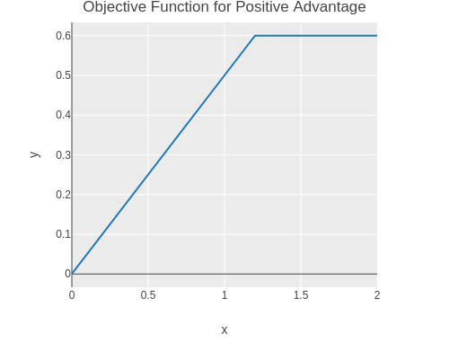
The objective is to increase the probability of actions which lead to a positive advantage and reduce the probability of actions which lead to a negative advantage.
I.e. maximising the following objective function.
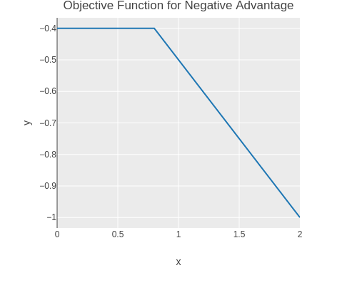
The core idea of PPO is to use clipped probability ratios for the loss function in order to increase stability, .
The probability ratio is clipped to stay below \(1+\epsilon\) for positive advantages and to stay above \(1-\epsilon\) for negative advantages.
Because PyTorch minimizes a loss, we need to negate above objective function.
(defnclipped-surrogate-loss"Clipped surrogate loss (negative objective)"[probability-ratiosadvantagesepsilon](torch/mean(torch/neg(torch/min(torch/mulprobability-ratiosadvantages)(torch/mul(torch/clampprobability-ratios(-1.0epsilon)(+1.0epsilon))advantages)))))
We can plot the objective function for a single action and a positive advantage.
(without-gradient(let[ratios(range0.02.010.01)loss(fn[ratioadvantageepsilon](toitem(torch/neg(clipped-surrogate-loss(tensorratio)(tensoradvantage)epsilon))))scatter(tc/dataset{:xratios:y(map(fn[ratio](lossratio0.50.2))ratios)})](->scatter(plotly/base{:=title"Objective Function for Positive Advantage":=mode:lines})(plotly/layer-point{:=x:x:=y:y}))))
And for a negative advantage.
(without-gradient(let[ratios(range0.02.010.01)loss(fn[ratioadvantageepsilon](toitem(torch/neg(clipped-surrogate-loss(tensorratio)(tensoradvantage)epsilon))))scatter(tc/dataset{:xratios:y(map(fn[ratio](lossratio-0.50.2))ratios)})](->scatter(plotly/base{:=title"Objective Function for Negative Advantage":=mode:lines})(plotly/layer-point{:=x:x:=y:y}))))
We can now implement the actor loss function which we want to minimize.
The loss function uses the clipped surrogate loss function as defined above.
The loss function also penalises low entropy values of the distributions output by the actor in order to encourage exploration.
(defnactor-loss"Compute loss value for batch of samples and actor"[samplesactorepsilonentropy-factor](let[ratios(probability-ratiossamples(logprob-of-actionactor))entropy(torch/mulentropy-factor(torch/neg(torch/mean(entropy-of-distributionactor(:observationssamples)))))surrogate-loss(clipped-surrogate-lossratios(:advantagessamples)epsilon)](torch/addsurrogate-lossentropy)))
A notable detail in XinJingHao’s PPO implementation is that the advantage values used in the actor loss (not in the critic loss!) are normalized.
The data required for training needs to be converted to PyTorch tensors.
(defntensor-batch"Convert batch to Torch tensors"[batch]{:observations(tensor(:observationsbatch)):logprobs(tensor(:logprobsbatch)):actions(tensor(:actionsbatch)):advantages(tensor(:advantagesbatch))})
Furthermore it is good practice to shuffle the samples.
This ensures that samples early and late in the sequence are not threated differently.
Note that you need to shuffle after computing the advantages, because the computation of the advantages relies on the order of the samples.
We separate the generation of random indices to facilitate unit testing of the shuffling function.
(defnrandom-order"Create a list of randomly ordered indices"[n](shuffle(rangen)))(defnshuffle-samples"Random shuffle of samples"([samples](shuffle-samplessamples(random-order(python/len(first(valssamples))))))([samplesindices](zipmap(keyssamples)(map#(torch/index_select%0(torch/tensorindices))(valssamples)))))
(defnsample-with-advantage-and-critic-target"Create batches of samples and add add advantages and critic target values"[environment-factoryactorcriticsizebatch-sizegammalambda](->>(sample-environmentenvironment-factory(indeterministic-actactor)size)(assoc-advantages(critic-observationcritic)gammalambda)tensor-batch(assoc-critic-targetcritic)normalize-advantagesshuffle-samples(create-batchesbatch-size)))
PPO Main Loop
Now we can implement the PPO main loop.
The outer loop samples the environment using the current actor (i.e. policy) and computes the data required for training.
The inner loop performs a small number of updates using the samples from the outer loop.
Each update step performs a gradient descent update for the actor and a gradient descent update for the critic.
Another detail from XinJingHao’s PPO implementation is that the gradient norm for the actor update is clipped.
At the end of the loop, the smoothed loss values are shown and the deterministic actions and entropies for a few observations are shown which helps with parameter tuning.
Furthermore the entropy factor is slowly lowered so that the policy reduces exploration over time.
The actor and critic model are saved to disk after each checkpoint.
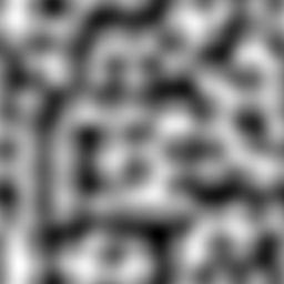
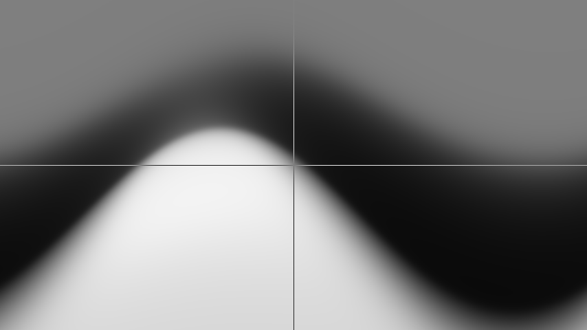
This image shows the motor control input as a function of pendulum angle and angular velocity.
As one can see, the pendulum is decelerated when the speed is high (dark values at the top of the image).
Near the centre of the image (speed zero and angle zero) one can see how the pendulum is accelerated when the angle is negative and the speed small and decelerated when the angle is positive and the speed is small.
Also the image is not symmetrical because otherwise the pendulum would not start swinging up when pointing downwards (left and right boundary of the image).
Automated Pendulum
The pendulum implementation can now be updated to use the actor instead of the mouse position as motor input when the mouse button is pressed.
(defn-main[&_args](let[actor(Actor3641)done-chan(async/chan)last-action(atom{:control0.0})](when(.exists(java.io.File."actor.pt"))(py.actorload_state_dict(torch/load"actor.pt")))(q/sketch:title"Inverted Pendulum with Mouse Control":size[854480]:setup#(setupPI0.0):update(fn[state](let[observation(observationstateconfig)action(if(q/mouse-pressed?)(action(tolist(py.actordeterministic_act(tensorobservation)))){:control(min1.0(max-1.0(-1.0(/(q/mouse-x)(/(q/width)2.0)))))})state(update-statestateactionconfig)](when(done?stateconfig)(async/close!done-chan))(reset!last-actionaction)state)):draw#(draw-state%@last-action):middleware[m/fun-mode]:on-close(fn[&_](async/close!done-chan)))(async/<!!done-chan))(System/exit0))
Here is a small demo video of the pendulum being controlled using the actor network.
You can find a repository with the code of this article as well as unit tests at github.com/wedesoft/ppo.
Then I tried the following program to train a neural network to imitate an XOR gate.
importtorchimporttorch.nnasnnimporttorch.optimasoptim# Check if GPU is available
device=torch.device("cuda"iftorch.cuda.is_available()else"cpu")# XOR data
X=torch.tensor([[0,0],[0,1],[1,0],[1,1]],dtype=torch.float32).to(device)Y=torch.tensor([[0],[1],[1],[0]],dtype=torch.float32).to(device)# Define the neural network
classXORNet(nn.Module):def__init__(self):super(XORNet,self).__init__()self.fc1=nn.Linear(2,5)self.fc2=nn.Linear(5,1)self.sigmoid=nn.Sigmoid()defforward(self,x):x=torch.relu(self.fc1(x))x=self.sigmoid(self.fc2(x))returnx# Initialize the network, loss function and optimizer
model=XORNet().to(device)criterion=nn.BCELoss()optimizer=optim.SGD(model.parameters(),lr=0.1)# Training loop
forepochinrange(10000):model.train()optimizer.zero_grad()outputs=model(X)loss=criterion(outputs,Y)loss.backward()optimizer.step()if (epoch+1)%1000==0:print(f'Epoch [{epoch+1}/10000], Loss: {loss.item():.4f}')# Test the model
model.eval()withtorch.no_grad():predictions=model(X)print("Predictions:",predictions.round())
However I got the following error (using Torch 2.9.1 and ROCm 7.2.0).
RuntimeError: CUDA error: HIPBLAS_STATUS_INVALID_VALUE when calling `hipblasLtMatmulAlgoGetHeuristic( ltHandle, computeDesc.descriptor(), Adesc.descriptor(), Bdesc.descriptor(), Cdesc.descriptor(), Cdesc.descriptor(), preference.descriptor(), 1, &heuristicResult, &returnedResult)`
To download the required libraries, we use a deps.edn file with the following content:
Replace the natives-linux classifier with natives-macos or natives-windows as required.
Here is a corresponding Midje test.
Note that ideally you practise Test Driven Development (TDD), i.e. you start with writing one failing test.
Because this is a Clojure notebook, the unit tests are displayed after the implementation.
We test the method by replacing the random function with a deterministic function.
(facts"Place random point in a cell"(with-redefs[rand(fn[s](*0.5s))](random-point-in-cell{:cellsize1}00)=>(vec20.50.5)(random-point-in-cell{:cellsize2}00)=>(vec21.01.0)(random-point-in-cell{:cellsize2}03)=>(vec27.01.0)(random-point-in-cell{:cellsize2}20)=>(vec21.05.0)(random-point-in-cell{:cellsize2}235)=>(vec311.07.05.0)))
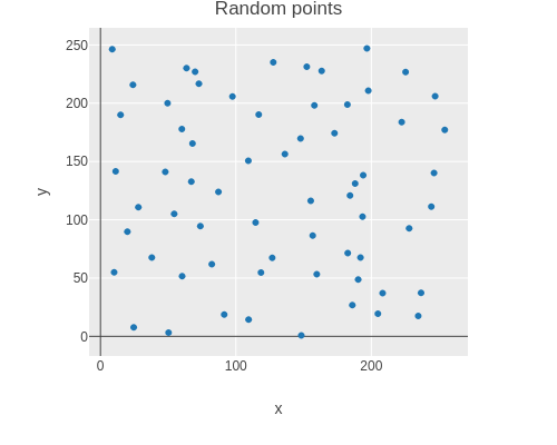
We can now use the random-point method to generate a grid of random points.
The grid is represented using a tensor from the dtype-next library.
(facts"Greate grid of random points"(let[params-2d(make-noise-params3282)params-3d(make-noise-params3283)](with-redefs[rand(fn[s](*0.5s))](dtype/shape(random-pointsparams-2d))=>[88]((random-pointsparams-2d)00)=>(vec22.02.0)((random-pointsparams-2d)03)=>(vec214.02.0)((random-pointsparams-2d)20)=>(vec22.010.0)(dtype/shape(random-pointsparams-3d))=>[888]((random-pointsparams-3d)235)=>(vec322.014.010.0))))
Here is a scatter plot showing one random point placed in each cell.
(facts"Wrap around components of vector to be within -size/2..size/2"(mod-vec{:size8}(vec223))=>(vec223)(mod-vec{:size8}(vec252))=>(vec2-32)(mod-vec{:size8}(vec225))=>(vec22-3)(mod-vec{:size8}(vec2-52))=>(vec232)(mod-vec{:size8}(vec22-5))=>(vec223)(mod-vec{:size8}(vec3231))=>(vec3231)(mod-vec{:size8}(vec3521))=>(vec3-321)(mod-vec{:size8}(vec3251))=>(vec32-31)(mod-vec{:size8}(vec3235))=>(vec323-3)(mod-vec{:size8}(vec3-521))=>(vec3321)(mod-vec{:size8}(vec32-51))=>(vec3231)(mod-vec{:size8}(vec323-5))=>(vec3233))
Using the mod-dist function we can calculate the distance between two points in the periodic noise array.
The tabular macro implemented by Midje is useful for running parametrized tests.
(tabular"Wrapped distance of two points"(fact(mod-dist{:size8}(vec2?ax?ay)(vec2?bx?by))=>?result)?ax?ay?bx?by?result00000.000202.000503.000022.000053.020002.050003.002002.005003.0)
Modular lookup
We also need to lookup elements with wrap around.
We recursively use tensor/select and then finally the tensor as a function to lookup along each axis.
A tensor with index vectors is used to test the lookup.
(facts"Wrapped lookup of tensor values"(let[t(tensor/compute-tensor[46]vec2)](wrap-gett23)=>(vec223)(wrap-gett27)=>(vec221)(wrap-gett53)=>(vec213)(wrap-get(wrap-gett5)3)=>(vec213)))
The following function converts a noise coordinate to the index of a cell in the random point array.
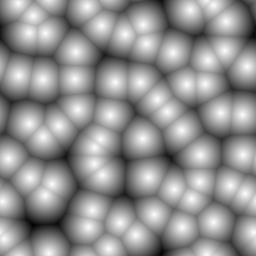
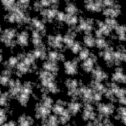
Using above functions one can now implement Worley noise.
For each pixel the distance to the closest seed point is calculated.
This is achieved by determining the distance to each random point in all neighbouring cells and then taking the minimum.
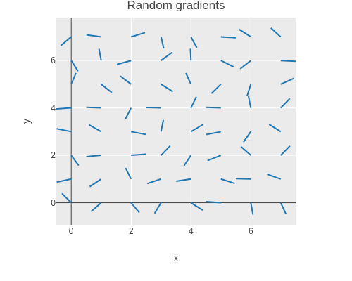
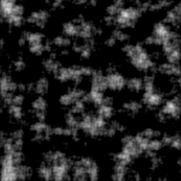
Perlin noise is generated by choosing a random gradient vector at each cell corner.
The noise tensor’s intermediate values are interpolated with a continuous function, utilizing the gradient at the corner points.
Random gradients
The 2D or 3D gradients are generated by creating a vector where each component is set to a random number between -1 and 1.
Random vectors are generated until the vector length is greater 0 and lower or equal to 1.
The vector then is normalized and returned.
Random vectors outside the unit circle or sphere are discarded in order to achieve a uniform distribution on the surface of the unit circle or sphere.
In the following tests, the random function is again replaced with a deterministic function.
(facts"Create unit vector with random direction"(with-redefs[rand(constantly0.5)](random-gradient00)=>(roughly-vec(vec2(-(sqrt0.5))(-(sqrt0.5)))1e-6))(with-redefs[rand(constantly1.5)](random-gradient00)=>(roughly-vec(vec2(sqrt0.5)(sqrt0.5))1e-6)))
The random gradient function is then used to generate a field of random gradients.
The next step is to determine the vectors to the corners of the cell for a given point.
First we define a function to determine the fractional part of a number.
(defnfrac[x](-x(Math/floorx)))(facts"Fractional part of floating point number"(frac0.25)=>0.25(frac1.75)=>0.75(frac-0.25)=>0.75)
This function can be used to determine the relative position of a point in a cell.
(defncell-pos[{:keys[cellsize]}point](applyvec-n(mapfrac(divpointcellsize))))(facts"Relative position of point in a cell"(cell-pos{:cellsize4}(vec223))=>(vec20.50.75)(cell-pos{:cellsize4}(vec275))=>(vec20.750.25)(cell-pos{:cellsize4}(vec3752))=>(vec30.750.250.5))
A 2 × 2 tensor of corner vectors can be computed by subtracting the corner coordinates from the point coordinates.
(facts"Compute relative vectors from cell corners to point in cell"(let[corners2(corner-vectors{:cellsize4:dimensions2}(vec276))corners3(corner-vectors{:cellsize4:dimensions3}(vec3765))](corners200)=>(vec20.750.5)(corners201)=>(vec2-0.250.5)(corners210)=>(vec20.75-0.5)(corners211)=>(vec2-0.25-0.5)(corners3000)=>(vec30.750.50.25)))
Extract gradients of cell corners
The function below retrieves the gradient values at a cell’s corners, utilizing wrap-get for modular access.
The result is a 2 × 2 tensor of gradient vectors.
(facts"Get 2x2 tensor of gradients from a larger tensor using wrap around"(let[gradients2(tensor/compute-tensor[46](fn[yx](vec2xy)))gradients3(tensor/compute-tensor[468](fn[zyx](vec3xyz)))]((corner-gradients{:cellsize4:dimensions2}gradients2(vec296))00)=>(vec221)((corner-gradients{:cellsize4:dimensions2}gradients2(vec296))01)=>(vec231)((corner-gradients{:cellsize4:dimensions2}gradients2(vec296))10)=>(vec222)((corner-gradients{:cellsize4:dimensions2}gradients2(vec296))11)=>(vec232)((corner-gradients{:cellsize4:dimensions2}gradients2(vec22315))11)=>(vec200)((corner-gradients{:cellsize4:dimensions3}gradients3(vec3963))000)=>(vec3210)))
Influence values
The influence value is the function value of the function with the selected random gradient at a corner.
(facts"Compute influence values from corner vectors and gradients"(let[gradients2(tensor/compute-tensor[22](fn[_yx](vec2x10)))vectors2(tensor/compute-tensor[22](fn[y_x](vec21y)))influence2(influence-valuesgradients2vectors2)gradients3(tensor/compute-tensor[222](fn[zyx](vec3xyz)))vectors3(tensor/compute-tensor[222](fn[_z_y_x](vec3110100)))influence3(influence-valuesgradients3vectors3)](influence200)=>0.0(influence201)=>1.0(influence210)=>10.0(influence211)=>11.0(influence3111)=>111.0))
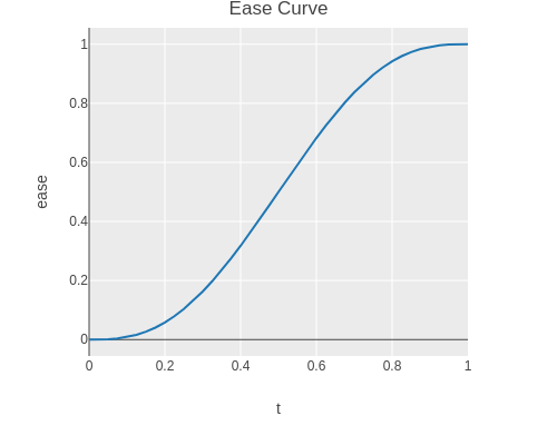
Interpolating the influence values
For interpolation the following “ease curve” is used.
(facts"Monotonously increasing function with zero derivative at zero and one"(ease-curve0.0)=>0.0(ease-curve0.25)=>(roughly0.1035161e-6)(ease-curve0.5)=>0.5(ease-curve0.75)=>(roughly0.8964841e-6)(ease-curve1.0)=>1.0)
The ease curve monotonously increases in the interval from zero to one.
Here x-, y-, and z-ramps are used to test that interpolation works.
(facts"Interpolate values of tensor"(let[x2(tensor/compute-tensor[46](fn[_yx]x))y2(tensor/compute-tensor[46](fn[y_x]y))x3(tensor/compute-tensor[468](fn[_z_yx]x))y3(tensor/compute-tensor[468](fn[_zy_x]y))z3(tensor/compute-tensor[468](fn[z_y_x]z))](interpolatex22.53.5)=>3.0(interpolatey22.53.5)=>2.0(interpolatex22.54.0)=>3.5(interpolatey23.03.5)=>2.5(interpolatex20.00.0)=>2.5(interpolatey20.00.0)=>1.5(interpolatex32.53.55.5)=>5.0(interpolatey32.53.53.0)=>3.0(interpolatez32.53.55.5)=>2.0))
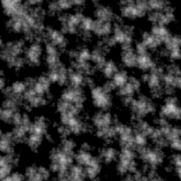
Octaves of noise
Fractal Brownian Motion is implemented by computing a weighted sum of the same base noise function using different frequencies.
(tabular"Remap values of tensor"(fact((remap(tensor/->tensor[?value])?low1?high1?low2?high2)0)=>?expected)?value?low1?high1?low2?high2?expected001010101011001232101233223010323011102042)
The clamp function is used to element-wise clamp values to a range.
In order to render the clouds we create a window and an OpenGL context.
Note that we need to create an invisible window to get an OpenGL context, even though we are not going to draw to the window
The following method creates a program and the quad VAO and sets up the memory layout.
The program and VAO are then used to render a single pixel.
Using this method we can write unit tests for OpenGL shaders!
We can test this mock function using the following probing shader.
Note that we are using the template macro of the comb Clojure library to generate the probing shader code from a template.
(defnoise-probe(template/fn[xyz]"#version 130
out vec4 fragColor;
float noise(vec3 idx);
void main()
{
fragColor = vec4(noise(vec3(<%= x %>, <%= y %>, <%= z %>)));
}"))
Here multiple tests are run to test that the mock implements a checkboard pattern correctly.
Again we use a probing shader to test the shader function.
(defoctaves-probe(template/fn[xyz]"#version 130
out vec4 fragColor;
float octaves(vec3 idx);
void main()
{
fragColor = vec4(octaves(vec3(<%= x %>, <%= y %>, <%= z %>)));
}"))
A few unit tests with one or two octaves are sufficient to drive development of the shader function.
(tabular"Test octaves of noise"(fact(first(render-pixel[vertex-passthrough][noise-mock(noise-octaves?octaves)(octaves-probe?x?y?z)]))=>?result)?x?y?z?octaves?result000[1.0]0.0100[1.0]1.0100[0.5]0.50.500[0.01.0]1.00.500[0.01.0]1.0100[1.00.0]1.0)
Shader for intersecting a ray with a box
The following shader implements intersection of a ray with an axis-aligned box.
The shader function returns the distance of the near and far intersection with the box.
The ray-box shader is tested with different ray origins and directions.
(tabular"Test intersection of ray with box"(fact((juxtfirstsecond)(render-pixel[vertex-passthrough][ray-box(ray-box-probe?ox?oy?oz?dx?dy?dz)]))=>?result)?ox?oy?oz?dx?dy?dz?result-200100[1.03.0]-200200[0.51.5]-222100[0.00.0]0-20010[1.03.0]0-20020[0.51.5]2-22010[0.00.0]00-2001[1.03.0]00-2002[0.51.5]22-2001[0.00.0]000100[0.01.0]200100[0.00.0])
Shader for light transfer through clouds
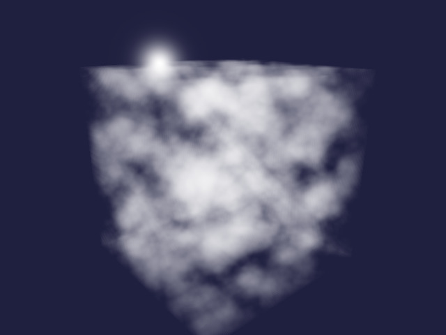
We test the light transfer through clouds using constant density fog.
The following fragment shader is used to render an image of a box filled with fog.
The pixel coordinate and the resolution of the image are used to determine a viewing direction which also gets rotated using the rotation matrix and normalized.
The origin of the camera is set at a specified distance to the center of the box and rotated as well.
The ray box function is used to determine the near and far intersection points of the ray with the box.
The cloud transfer function is used to sample the cloud density along the ray and determine the overall opacity and color of the fog box.
The background is a mix of blue color and a small blob of white where the viewing direction points to the light source.
The opacity value of the fog is used to overlay the fog color over the background.
Uniform variables are parameters that remain constant throughout the shader execution, unlike vertex input data.
Here we use the following uniform variables:
resolution: a 2D vector containing the window pixel width and height
light: a 3D unit vector pointing to the light source
rotation: a 3x3 rotation matrix to rotate the camera around the origin
focal_length: the ratio of camera focal length to pixel size of the virtual camera
The following function sets up the shader program, the vertex array object, and the uniform variables.
Then GL11/glDrawElements draws the background quad used for performing volumetric rendering.
We also need to convert the floating point array to a tensor and then to a BufferedImage.
The one-dimensional array gets converted to a tensor and then reshaped to a 3D tensor containing width × height RGBA values.
The RGBA data is converted to BGR data and then multiplied with 255 and clamped.
Finally the tensor is converted to a BufferedImage.
Finally we are ready to render the volumetric fog.
(rgba-array->bufimg(render-fog640480)640480)
Rendering of 3D noise
This method converts a floating point array to a buffer and initialises a 3D texture with it.
It is also necessary to set the texture parameters for interpolation and wrapping.
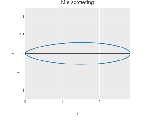
In-scattering of light towards the observer depends of the angle between light source and viewing direction.
Here we are going to use the phase function by Cornette and Shanks which depends on the asymmetry g and mu = cos(theta).
(defmie-scatter(template/fn[g]"#version 450 core
#define M_PI 3.1415926535897932384626433832795
#define ANISOTROPIC 0.25
#define G <%= g %>
uniform vec3 light;
float mie(float mu)
{
return 3 * (1 - G * G) * (1 + mu * mu) /
(8 * M_PI * (2 + G * G) * pow(1 + G * G - 2 * G * mu, 1.5));
}
float in_scatter(vec3 point, vec3 direction)
{
return mix(1.0, mie(dot(light, direction)), ANISOTROPIC);
}"))
We define a probing shader.
(defmie-probe(template/fn[mu]"#version 450 core
out vec4 fragColor;
float mie(float mu);
void main()
{
float result = mie(<%= mu %>);
fragColor = vec4(result, 0, 0, 1);
}"))
The shader is tested using a few values.
(tabular"Shader function for scattering phase function"(fact(first(render-pixel[vertex-passthrough][(mie-scatter?g)(mie-probe?mu)]))=>(roughly?result1e-6))?g?mu?result00(/3(*16PI))01(/6(*16PI))0-1(/6(*16PI))0.50(/(*30.75)(*8PI2.25(pow1.251.5)))0.51(/(*60.75)(*8PI2.25(pow0.251.5))))
We can define a function to compute a particular value of the scattering phase function using the GPU.
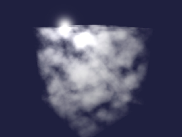
Finally we can implement the shadow function by also sampling towards the light source to compute the shading value at each point.
Testing the function requires extending the render-pixel function to accept a function for setting the light uniform.
We leave this as an exercise for the interested reader 😉.
(defshadow(template/fn[noisestep]"#version 130
#define STEP <%= step %>
uniform vec3 light;
float <%= noise %>(vec3 idx);
vec2 ray_box(vec3 box_min, vec3 box_max, vec3 origin, vec3 direction);
float shadow(vec3 point)
{
vec2 interval = ray_box(vec3(-0.5, -0.5, -0.5), vec3(0.5, 0.5, 0.5), point, light);
float result = 1.0;
for (float t = interval.x + 0.5 * STEP; t < interval.y; t += STEP) {
float density = <%= noise %>(point + t * light);
float transmittance = exp(-density * STEP);
result *= transmittance;
};
return result;
}"))


 This image shows the motor control input as a function of pendulum angle and angular velocity.
As one can see, the pendulum is decelerated when the speed is high (dark values at the top of the image).
Near the centre of the image (speed zero and angle zero) one can see how the pendulum is accelerated when the angle is negative and the speed small and decelerated when the angle is positive and the speed is small.
Also the image is not symmetrical because otherwise the pendulum would not start swinging up when pointing downwards (left and right boundary of the image).
This image shows the motor control input as a function of pendulum angle and angular velocity.
As one can see, the pendulum is decelerated when the speed is high (dark values at the top of the image).
Near the centre of the image (speed zero and angle zero) one can see how the pendulum is accelerated when the angle is negative and the speed small and decelerated when the angle is positive and the speed is small.
Also the image is not symmetrical because otherwise the pendulum would not start swinging up when pointing downwards (left and right boundary of the image).