Rigid body game physics 2
13 Nov 2019part 1 part 2 part 3 part 4 part 5 part 6
Update: See Getting started with the Jolt Physics Engine
The following article is heavily based on Hubert Eichner’s article on equality constraints. The math for the joint types was taken from Kenny Erleben’s PhD thesis.
Constraint Impulses
A constraint between two objects is specified as a multi-dimensional function C(y(t)).
The constrained is fulfilled by attempting to keep each component of the derivative of C at zero:
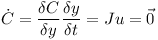 J is the Jacobian matrix and u is a twelve-element vector containing the linear and rotational speed of the two bodies.
Here the derivative of the orientation is represented using the rotational speed ω.
J is the Jacobian matrix and u is a twelve-element vector containing the linear and rotational speed of the two bodies.
Here the derivative of the orientation is represented using the rotational speed ω.
 The two objects without a connecting joint would together have twelve degrees of freedom.
Let’s assume that the two objects are connected by a hinge joint.
In this case the function C has five dimensions because a hinge only leaves seven degrees of freedom.
The Jacobian J has five rows and twelve columns.
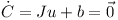
In practise an additional vector b is used to correct for numerical errors.
The two objects without a connecting joint would together have twelve degrees of freedom.
Let’s assume that the two objects are connected by a hinge joint.
In this case the function C has five dimensions because a hinge only leaves seven degrees of freedom.
The Jacobian J has five rows and twelve columns.
In practise an additional vector b is used to correct for numerical errors.
The twelve-element constraint impulse P does not do any work and therefore must be orthogonal to u.
 The rows of J span the orthogonal space to u. Therefore P can be expressed as a linear combination of the rows of J
 where λ is a vector with for example five elements in the case of the hinge joint.
Given an initial estimate for u and the constraint impulse P one can compute the final velocity u.
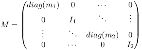
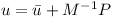 M is the twelve by twelve generalised mass matrix which contains the mass and inertia tensors of the two objects.
 Inserting the equation for u into the constraint equation yields
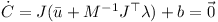 This equation can be used to determine λ
 λ then can be used to determine the constraint impulse P!
When performing the numerical integration, the external forces (multiplied with the timestep) and the constraint impulse are used
to determine the change in linear and rotational speed of the two bodies.
λ then can be used to determine the constraint impulse P!
When performing the numerical integration, the external forces (multiplied with the timestep) and the constraint impulse are used
to determine the change in linear and rotational speed of the two bodies.
Joints
Ball-in-Socket Joint
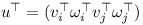
The matrix J for bodies i and j and the velocity vector u can be split up into the linear and angular parts.
 v is the three-dimensional linear speed and ω is the rotational speed of the individual object.
At the anchor point of the joint the speed of the two rigid bodies must be the same:
v is the three-dimensional linear speed and ω is the rotational speed of the individual object.
At the anchor point of the joint the speed of the two rigid bodies must be the same:
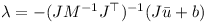
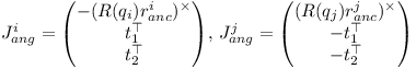
 Thus the linear components of J are
 and the angular components of J are
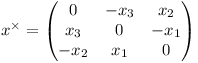
 where the cross-product matrix of a vector is defined as follows:
 The correcting vector b simply corrects for the offset at the anchor point.

Hinge Joint
A hinge joint has the constraints of the ball-in-socket joint and two additional angular constraints.
I.e. there are five constraints altogether.
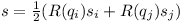
 The rotation axis in world coordinates can be computed from the average of the two rotated axes
which should be coinciding under ideal circumstances.
The rotation axis in world coordinates can be computed from the average of the two rotated axes
which should be coinciding under ideal circumstances.
The relative rotation of the two rigid bodies must be parallel to the axis s of the hinge.
Given two vectors t1 and t2 orthogonal to the rotation axis of the hinge joint,
the two additional constraints are:
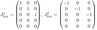
 Therefore the angular parts of the Jacobian are
The error u of axis misalignment is the cross product of the two rotated axes.
 The error u is orthogonal to the rotation axis s.
It is projected onto the vectors t1 and t2 when computing the correction vector b:
The error u is orthogonal to the rotation axis s.
It is projected onto the vectors t1 and t2 when computing the correction vector b:

See Kenny Erleben’s PhD thesis for these and other types of joints (slider joint, hinge-2 joint, universal joint, fixed joint).
Sequential Impulses
To fulfill multiple constraints, an algorithm called sequential impulses is used. Basically the constraint impulses are updated a few times until the impulses become stable.
- for each iteration
- for each joint
- compute Jacobian J and correction vector b
- predict speed u
- compute λ
- compute the impulse P
- add P to accumulated impulses of the two objects
- for each joint
- use impulses and external forces to perform Runge Kutta integration step
The sequential impulse iterations have to be performed four times when using the Runge-Kutta method.