25 Nov 2019
part 1
part 2
part 3
part 4
part 5
part 6
Update: See Getting started with the Jolt Physics Engine
The following article is based on Hubert Eichner’s article on inequality constraints.
Contact points (resting contacts) are represented as inequality constraints.
In contrast to a joint, a resting contact can only create repellent forces and no attracting forces.
Similar to a joint constraint, the resting contact is represented using a function C(y(t)).
Here C is one-dimensional and it is basically the distance of the two objects at the contact point.
The inequality constraint of the resting contact is
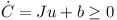 with the matrix J having one row and twelve columns.
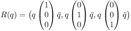
Instead of anchor points, one uses vectors ri and rj from the center of each object to the contact point.
Using the contact normal n the inequality constraint becomes:
with the matrix J having one row and twelve columns.
Instead of anchor points, one uses vectors ri and rj from the center of each object to the contact point.
Using the contact normal n the inequality constraint becomes:
 The rotational component can be simplified as shown below:
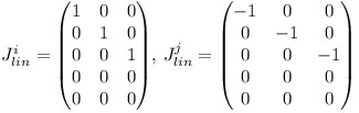
 Thus the linear components of J are
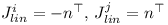 And the angular components of J are
 The correction term depends on the distance d.
I.e. if the distance is negative, a correction is required so that the objects do not penetrate each other any more.
The correction term depends on the distance d.
I.e. if the distance is negative, a correction is required so that the objects do not penetrate each other any more.

Sequential Impulses (updated)
The impulses generated by contact constraints and joint constraints are accumulated in a loop.
The (cumulative) λ obtained for contact constraint furthermore is clipped to be greater or equal to zero.
Note that it has to be the cumulative value which is clipped.
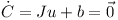
The algorithm for solving the joint and contact constraints becomes:
- for each iteration
- for each joint
- compute Jacobian J and correction vector b
- predict speed u
- compute λ
- compute the impulse P
- add P to accumulated impulses of the two objects
- for each resting contact
- subtract old impulses P from previous iteration from accumulated impulses of the two objects
- compute Jacobian J and correction vector b
- predict speed u
- compute new λ and clip it to be greater or equal to zero
- compute the impulse P
- add P to accumulated impulses of the two objects
- use impulses and external forces to perform Runge Kutta integration step
The sequential impulse iterations have to be performed four times when using the Runge-Kutta method.
The value λ is stored as Pn for limiting friction impulses lateron.

24 Oct 2019
part 1
part 2
part 3
part 4
part 5
part 6
Update: See Getting started with the Jolt Physics Engine
Inspired by Hubert Eichner’s articles on game physics I decided to write about rigid body dynamics as well.
My motivation is to create a space flight simulator.
Hopefully it will be possible to simulate a space ship with landing gear and docking adapter using multiple rigid bodies.
The Newton-Euler equation
Each rigid body has a center with the 3D position c.
The orientation of the object can be described using a quaternion q which has four components.
The speed of the object is a 3D vector v.
Finally the 3D vector ω specifies the current rotational speed of the rigid body.
The time derivatives (indicated by a dot on top of the variable name) of the position and the orientation are (Sauer et al.):
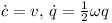 The multiplication is a quaternion multiplication where the rotational speed ω is converted to a quaternion:

In a given time step Δt the position changes as follows
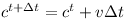
The orientation q changes as shown below
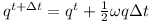 Note that ω again is converted to a quaternion.
Given the mass m and the sum of external forces F the speed changes like this
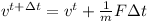 In other words this means

Finally given the rotated inertia matrix I(t) and the overall torque τ one can determine the change of rotational speed
 Or written as a differential equation
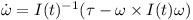
These are the Newton-Euler equations.
The “x” is the vector cross product.
Note that even if the overall torque τ is zero, the rotation vector still can change over time if the inertial matrix I has different eigenvalues.
The rotated inertia matrix is obtained by converting the quaternion q to a rotation matrix R and using it to rotate I₀:
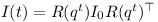
The three column vectors of R can be determined by performing quaternion rotations on the unit vectors.
 Note that the vectors get converted to quaternion and back implicitely.
According to David Hammen, the Newton-Euler equation can be used unmodified in the world inertial frame.
The Runge-Kutta Method
The different properties of the rigid body can be stacked in a state vector y as follows.
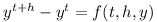
 The equations above then can be brought into the following form
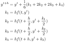
 Using h=Δt the numerical integration for a time step can be performed using the Runge-Kutta method:
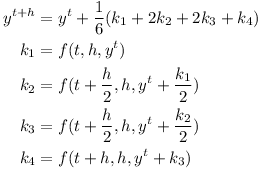
The Runge-Kutta algorithm can also be formulated using a function which instead of derivatives returns infitesimal changes
The Runge-Kutta formula then becomes
Using time-stepping with F=0 and τ=0 one can simulate an object tumbling in space.
06 May 2019
A GRU and a fully connected layer with softmax output can be used to recognise words in an audio stream (sequence to sequence).
I recorded a random sequence of 100 utterances of 4 words (“left”, “right”, “stop”, “go”) with a sampling rate of 11025Hz.
Furthermore 300 seconds of background noise were recorded.
All audio data was grouped into chunks of 512 samples.
The logarithm of the Fourier spectrum of each chunk was used as input for the GRU.
The initial state of the GRU (128 units) was set to zero.
The network was trained in a sequence-to-sequence setting to recognise words given a sequence of audio chunks.

The example was trained using gradient descent with learning rate alpha = 0.05.
The background noise was cycled randomly and words were inserted with random length pause between them.
The network was trained to output the word label 10 times after recognising a word.
The training took about one hour on a CPU.
The resulting example is more minimalistic than the Tensorflow audio recognition example.
The algorithm is very similar to an exercise in Andrew Ng’s Deep learning specialization.
Update:
See CourseDuck for a curated list of machine learning online courses.
27 Jan 2019
An LSTM can be used to recognise words from audio data (sequence to one).
I recorded a random sequence of 320 utterances of 5 words (“left”, “right”, “stop”, “go”, and “?” for background noise) with a sampling rate of 16kHz.
The audio data was split into chunks of 512 samples.
The word start and end were identified using a rising and a falling threshold for the root-mean-square value of each chunk.
The logarithm of the Fourier spectrum of each chunk was used as input for the LSTM.
The initial state and output of the LSTM (16 units each) was set to zero.
The final output state of the LSTM was used as input for a fully connected layer with 5 output units followed by a softmax classifier.
The network was trained in a sequence-to-one setting to recognise a word given a sequence of audio chunks as shown in the following figure.

The example was trained using gradient descent with multiplier alpha = 0.001.
The training took seven hours on a CPU.
The sequence-to-one setting handles words of different lengths gracefully.
The resulting example is more minimalistic than the Tensorflow audio recognition example.
In the following video the speech recognition is used to control a robot.
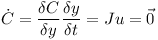 J is the Jacobian matrix and u is a twelve-element vector containing the linear and rotational speed of the two bodies.
Here the derivative of the orientation is represented using the rotational speed ω.
J is the Jacobian matrix and u is a twelve-element vector containing the linear and rotational speed of the two bodies.
Here the derivative of the orientation is represented using the rotational speed ω.
 The two objects without a connecting joint would together have twelve degrees of freedom.
Let’s assume that the two objects are connected by a hinge joint.
In this case the function C has five dimensions because a hinge only leaves seven degrees of freedom.
The Jacobian J has five rows and twelve columns.
In practise an additional vector b is used to correct for numerical errors.
The two objects without a connecting joint would together have twelve degrees of freedom.
Let’s assume that the two objects are connected by a hinge joint.
In this case the function C has five dimensions because a hinge only leaves seven degrees of freedom.
The Jacobian J has five rows and twelve columns.
In practise an additional vector b is used to correct for numerical errors.
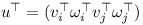
 The rows of J span the orthogonal space to u. Therefore P can be expressed as a linear combination of the rows of J
 where λ is a vector with for example five elements in the case of the hinge joint.
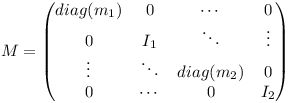
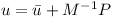 M is the twelve by twelve generalised mass matrix which contains the mass and inertia tensors of the two objects.
 Inserting the equation for u into the constraint equation yields
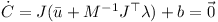 This equation can be used to determine λ
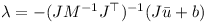 λ then can be used to determine the constraint impulse P!
When performing the numerical integration, the external forces (multiplied with the timestep) and the constraint impulse are used
to determine the change in linear and rotational speed of the two bodies.
λ then can be used to determine the constraint impulse P!
When performing the numerical integration, the external forces (multiplied with the timestep) and the constraint impulse are used
to determine the change in linear and rotational speed of the two bodies. v is the three-dimensional linear speed and ω is the rotational speed of the individual object.
At the anchor point of the joint the speed of the two rigid bodies must be the same:
v is the three-dimensional linear speed and ω is the rotational speed of the individual object.
At the anchor point of the joint the speed of the two rigid bodies must be the same:
 Thus the linear components of J are
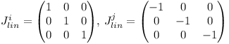 and the angular components of J are
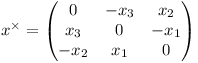
 where the cross-product matrix of a vector is defined as follows:
 The correcting vector b simply corrects for the offset at the anchor point.

 The rotation axis in world coordinates can be computed from the average of the two rotated axes
which should be coinciding under ideal circumstances.
The rotation axis in world coordinates can be computed from the average of the two rotated axes
which should be coinciding under ideal circumstances.
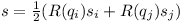
 Therefore the angular parts of the Jacobian are
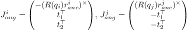
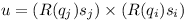 The error u is orthogonal to the rotation axis s.
It is projected onto the vectors t1 and t2 when computing the correction vector b:
The error u is orthogonal to the rotation axis s.
It is projected onto the vectors t1 and t2 when computing the correction vector b:
